My Youtube Channel

Please Subscribe

Flag of Nepal

Built in OpenGL

Word Cloud in Python

With masked image

Showing posts with label Machine learning. Show all posts

Wednesday, December 7, 2022

N-grams for text processing


N-gram is an N sequence of words. It can be a unigram (one word), bigram (sequence of two words), trigram (sequence of three words), and so on. It focuses on a sequence of words. Such a method is very useful in speech recognition and predicting input text. It helps us to predict the next words that could occur in a given sequence. Search engines also use the n-gram technique to predict the next word while a search query is typed in a search bar. 

Let us consider a sentence: 

This is going to be an amazing experience.


Unigram for the above sentence can be written as:
  • "This"
  • "is"
  • "going"
  • "to"
  • "be"
  • "an"
  • "amazing"
  • "experience"

Bigram for the above sentence can be written as:

  • “This is”
  • “is going”
  • “going to”
  • "to be"
  • "be an"
  • "an amazing"
  • "amazing experience"

Trigram for the above sentence can be written as:

  • "This is going"
  • "is going to "
  • "going to be"
  • "to be an"
  • "be an amazing"
  • "an amazing experience"

With n-grams, we can use a bag of n-grams (for example, a bag of bigrams) instead of only using a bag of words. A bag of bigrams or trigrams is more powerful than using just a bag of words as it takes the context into consideration as well.


Tuesday, December 6, 2022

Word embedding techniques for text processing

 It is difficult to perform analysis on the text so we use word embedding techniques to convert the texts into numerical representation. This is also called vectorization of the words. It is a representation technique for text in which words having same meaning are given similar representation. It helps to extract features from the text.

i. Bag of Words (BoW)

It is one of the most widely used technique for word embedding. This method focuses on the frequency of the words. It is easy to implement and also efficient at the same time.  In Python, we can use CountVectorizer() function from sklearn library to implement Bag of Words. A graphical representation of bag of Words has been shown in the figure below.

The reason for selecting BoW as word embedding technique is that it is still widely used technique due to its simplicity in implementation. It is also very useful when working on a domain specific dataset. If not entirely, it does give some idea to the researchers regarding the performance of the work.NLP: Bag of words and TF-IDF explained! | by Koushik kumar | Medium

 Fig: Representation of BoW


ii. TF-IDF (Term Frequency- Inverse Document Frequency)

Term Frequency is used to count the number of words in a document. It is not necessary that the words with higher frequencies tend to represent significant information about the document. A word appearing in a document for many times does not mean it is relevant and significant all the time. Many times, words with less frequencies carry more significant meanings about the document. One way to normalize the frequency of words is to use TF-IDF. Inverse Document Frequency (IDF) is used to calculate the significance of rare words or words with less frequencies.

The reason for using TF-IDF is it can be used to find and remove stop words in the textual data. It helps to find unique identifier in a text. It helps to understand the importance of a words in entire document which in turn can help in text summarization.


Easy understanding of Confusion matrix with examples

Confusion matrix is an important metric to evaluate the performance of classifier. The performance of a classifier depends on their capability predict the class correctly against new or unseen data. It is one of the easiest metrics for finding the correctness and accuracy of the model. The confusion matrix in itself is not a performance measure but all the performance metrics are based on confusion matrix. The ideal situation for any classification model would be when FP=0 and FN=0 but that’s not the case in real life. Depending upon the situation, we might want to minimize either FP or FN. 


Fig 3.10 Confusion Matrix


Let us consider both the situations with the help of example.

Case 1: Minimizing FN

Let,

1 = person having cancer

0 = person not having cancer

In this case, having some False Positive (FP) cases might be okay because classifying a non-cancerous person as cancerous does not affect a lot because on further test we will anyway find out that the particular person does not have cancer. But having False Negative (FN) cases can be hazardous because classifying a cancerous person as non-cancerous can cause serious threat to the life of that person. So, in this case we need to minimize FN.


Case 2: Minimizing FP

Let,

1 = Email is a spam

0 = Email is not spam

In this situation, having False Positive (FP) cases i.e., wrongly classifying non-spam or important email as spam can cause serious damage to the business, financial loss to the individuals and so on. Thus, in this situation we need to minimize FP.

Various metrics based on confusion matrix

  1. Accuracy: It is the number of correct predictions made by the model over all kinds of predictions made. It is a good measure when the target variable classes in the data are nearly balanced.


Accuracy = (TP+TN)/(TP+FP+TN+FN)


  1. Precision: It is defined as the ratio of number of positive samples correctly classified as positive to the total number of samples classified as positive (either correctly or incorrectly). It reflects how reliable the model is in classifying the samples as positive. It is used if the problem is sensitive to classifying a sample as positive in general.


Precision = TP/(TP+FP)


  1. Recall or sensitivity: It is defined as the ratio of number of positive samples correctly classified as positive to the total number of actual positive samples. It measures the model’s ability to detect positive samples. Higher the recall value, more positive samples are detected. It is independent of how the negative samples are classified. It is used if the goal is to detect all the positive samples without caring whether the negative samples would be misclassified as positive.


Recall = TP/(TP+FN)


Topic Modeling: Working of LSA (Latent Semantic Analysis) in simple terms

 LSA (Latent Semantic Analysis) is another technique used for topic modeling. The main concept behind topic modeling is that the meaning behind any document is based on some latent variables so we use various topic modeling techniques to unravel those hidden variables i.e., topics so that we can make sense of the given document. LSA is mostly suitable for large sets of documents. It converts the documents into a document term matrix before actually deriving topics from the documents.

Working of LSA:

  • The given text is converted into the document-term matrix using either bag of words or the Term Frequency- Inverse Document Frequency.

  • Then, using Truncated Singular Value Decomposition (SVD). It is at this stage the topics within the documents are identified. Mathematically, it can be given as,


Though it may look difficult to understand at first glance, in simple terms what the above formula represents is that it simply decomposes a high dimensional matrix into smaller matrices i.e., u, s, and v, where,

A = n*m document-term matrix (n = no. of documents and m = no. of words)

U = n*r document-topic matrix (n = no. of documents and r = no. of topics)

S = r*r matrix (r = no. of topics)

V = m*r word-topic matrix (m = no. of words and r = no. of topics)

  • Finally, we can now classify which document belongs to which topics.


Topic Modeling using Latent Semantic Analysis

Schematic diagram of LSA algorithm


Bi-LSTM in simple words

 In traditional neural networks, inputs and outputs were independent of each other. To predict next word in a sentence, it is difficult for such model to give correct output, as previous words are required to be remembered to predict the next word. For example, to predict the ending of a movie, it depends on how much one has already watched the movie and what contexts have arrived to that point of time in the movie. In the same way, RNN remembers everything. It overcomes the shortcomings of traditional neural network with the help of hidden layers. Because of the quality to remember the previous inputs, it useful in prediction of time series. This is called Long Short-Term Memory (LSTM).


Fig: LSTM Architecture


Combining two independent RNN together forms a Bi-LSTM (Bidirectional Long Short-Term Memory). It allows the network to have both forward and backward information. Bi-LSTM gives better result as it takes the context into consideration.

Example:

In NLP, to find the next word, it is not that we need only the previous word but also the upcoming word. As shown in the example above, to predict what comes after the word “Teddy”, we can’t be dependent only upon the previous word (which is “said” in this case) because it same in both the cases. Here, we need to consider the context as well. If we predict “Roosevelt” in the first case then it will be out of context as it will read as [He said, “Teddy Roosevelt are on sale!”]. So, Bi-LSTM is important to taken context into consideration.

Fig: Bi-LSTM Architecture


Topic Modeling

 Topic modeling is an unsupervised technique as it is used to perform analysis on text data having no label attached to it. As the name suggests, it is used to discover a number of topics within the given sets of text like tweets, books, articles, and so on. Each topic consists of words where the order of the words does not matter. It performs automatic clustering of words that best describe a set of documents. It gives us insight into a number of issues or features users are talking about, as a group. 

Topic Modelling With LDA -A Hands-on Introduction - Analytics Vidhya

For example, let us say a company has launched the software in the market and receives a number of feedback regarding various product features within a specified time period. Now, rather than going through each review one by one, if we apply topic modeling, we will come to know how users have perceived the various features of the product very quickly. It is one of the essential techniques to perform text analysis on unstructured data. After performing topic modeling, we can even perform topic classification to predict under which topic the upcoming reviews fall. There are various techniques to perform topic modeling, among which LDA is considered to be the most effective one.


Challenges of Sentiment analysis


  • Lack of availability of enough domain-specific dataset

  • Multi-class classification of the data

  • Difficult to extract the context of the post made by the users

  • Handling of neutral posts

  • Analyzing the posts of multiple languages

Saturday, November 28, 2020

Visualizing Decision tree in Python (with codes included)

List of libraries required to be installed (if not already installed). Here installation is done through Jupyter Notebook. For terminal use only "pip install library-name".

#import sys

#!{sys.executable} -m pip install numpy

#!{sys.executable} -m pip install pandas

#!{sys.executable} -m pip install sklearn

#!{sys.executable} -m pip install hvplot

#!{sys.executable} -m pip install six

#!{sys.executable} -m pip install pydotplus

#!{sys.executable} -m pip install  python-graphviz

Importing libraries:

import numpy as np 

import pandas as pd

from sklearn.tree import DecisionTreeClassifier

from sklearn import tree

import hvplot.pandas

About the dataset

Imagine that you are a medical researcher compiling data for a study. You have collected data about a set of patients, all of whom suffered from the same illness. During their course of treatment, each patient responded to one of 5 medications, Drug A, Drug B, Drug c, Drug x and y.

Part of your job is to build a model to find out which drug might be appropriate for a future patient with the same illness. The feature sets of this dataset are Age, Sex, Blood Pressure, and Cholesterol of patients, and the target is the drug that each patient responded to.

It is a sample of binary classifier, and you can use the training part of the dataset to build a decision tree, and then use it to predict the class of a unknown patient, or to prescribe it to a new patient.

Let's see the sample of dataset:

The shape of dataset is (200,6)

Pre-processing

Using my_data as the Drug.csv data read by pandas, declare the following variables:

  • as the Feature Matrix (data of my_data)
  • as the response vector (target)
  • Remove the column containing the target name since it doesn't contain numeric values.

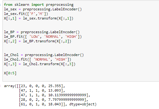
As you may figure out, some features in this dataset are categorical such as Sex or BP. Unfortunately, Sklearn Decision Trees do not handle categorical variables. But still we can convert these features to numerical values. pandas.get_dummies() Convert categorical variable into dummy/indicator variables.

Now we can fill the target variable.


Setting up the Decision Tree


We will be using train/test split on our decision tree. Let's import train_test_split from sklearn.cross_validation.


from sklearn.model_selection import train_test_split


Now train_test_split will return 4 different parameters. We will name them:
X_trainset, X_testset, y_trainset, y_testset

The train_test_split will need the parameters:
X, y, test_size=0.3, and random_state=3.

The X and y are the arrays required before the split, the test_size represents the ratio of the testing dataset, and the random_state ensures that we obtain the same splits.


Modeling


We will first create an instance of the DecisionTreeClassifier called drugTree.
Inside of the classifier, specify criterion="entropy" so we can see the information gain of each node.

We can use "gini" criterion as well. Result will be the same. Gini is actually a default criteria for decision tree classifier.


From the graph below, we can see the accuracy score is highest at max-depth=4 and it remains constant

thereafter so we have used max-depth=4 in this case.


We can also plot max-depth vs accuracy score for both testset and trainset:

For testset:


For trainset:


Now, plotting the graph of max-depth vs accuracy score for both trainset and testset:


Visualization


The final image of decision tree is given below:


Another easy method to generate decision tree:


Drawing Decision path (more readable form of decision tree):


Important features for classification

Listing the features in their rank of importance for classifying the data.


The github link to the program can be found here.

Sunday, August 16, 2020

Web scrapping using a single line of code in python

We will scrap the data of wikipedia using a single line of code in python. No extra libraries are required. Only Pandas can do the job.

Step 1: Install and import pandas library

import numpy as np 

Step 2: Read the data of web (here Wikipedia website) using pd.read_html('Website link here')[integer]

df = pd.read_html('https://en.wikipedia.org/wiki/COVID-19_pandemic_by_country_and_territory')[1]

Step 3: View the data scrapped from the web

Step 4: In case there are multiple table within a web page, you can change the index value to an integer starting from 0 until you get your required data (i.e. [0] or [1] or [2] or [3] and so on).

Build a colorful Word Cloud in python using mask image

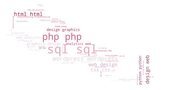
Word cloud is a data visualization tool in data science. It is very efficient to visualize various words in a text according to the quantum of their repetition within the text. The stopwords have been ignored while visualization. A text file called "skill.txt" has been used to visualize. Mask image of map of Nepal has been used to visualize the word cloud.

The libraries required are:

Reading the text file "alice.txt" whose word cloud will be formed. After reading text file, setting the stopwords.


Generating a word cloud and storing it into "skillwc" variable.

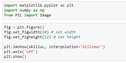
Importing libraries and creating a simple image of word cloud (without using mask image).


Now, using mask image of map of Nepal to create word cloud. First of all, we will open the image and save it in a variable "mask_image" and then view the mask image without superimposing the text onto it.


Click here to download the collection of mask image.

Finally, we will impose the text file 'alice.txt' onto the image shown above with adding original color of image to the word cloud instead of default color.


Get the Github link here.

Friday, August 14, 2020

Covid-19 Data Visualization across the World using Choropleth map

Introduction

This project visualizes the Covid-19 data (i.e. Total cases, Deaths and Recoveries) across various Provinces and Districts of Nepal as of 12th August, 2020. Geojson file of Nepal's states and districts have been used. Also python library i.e. Folium has been used to generate Choropleth map whose geo_data value is the geojson of Nepal.
The libraries imported are:

Data description:

Covid-19 data of  Countries across the world were scrapped from wikipedia.

Click here to go to the wikipedia page.

Simple one line code can be used to scrap the table of wikipedia. We will store the scrapped data into a dataframe called 'df'.

df = pd.read_html('https://en.wikipedia.org/wiki/COVID-19_pandemic_by_country_and_territory')[1]

View of original data:

Data Wrangling/ Cleaning:

Step 1: 

Selecting only required columns into new dataframe df1 from the data above.


Step 2:

 Converting the multi-index column into single-index colums.

Step 3:

Removing the index attached with the name of each countries in the dataframe above.

df1['Countries'] = df1['Countries'].str.replace(r'\[.*?\]$', '') 

Step 4:

Changing the country name 'United States' to 'United States of America' to match with the name in Geojson file.

df1['Countries'].replace('United States', 'United States of America', inplace=True)

Step 5:

We can see the last 3 rows of dataframe are not required so dropping them out.

df1=df1[:-3]

Step 6:

Replacing the value 'No data' to 0 (Zero) in each column.

df1['Recovered'].replace('No data', '0', inplace=True)


Step 7:

Changing the data type of columns Cases, Recovered and Deaths to integer.

After changing the datatypes:

Visualizing the data across world:

For cases:


Similarly, it can be done for Recovered and Deaths.

For recovered:

For deaths:


Get the Github link here.